Constrained Optimization Techniques

Provided by James R. Martin, Ph.D., CMA
Professor Emeritus, University of South Florida

Contsrained Optimization Controversy Main Page | Graduate MA Course

What is Constrained Optimization?

Constrained optimization models are based on a set of underlying assumptions. The main assumption is that most, if not all, of the various constraints in the model are static. The general idea is to find the optimum solution given a set of static constraints. Most of the models in accounting, finance, management, economics and quantitative methods fall into this category and can be criticized from the continuous improvement perspective (e.g., Deming's theory, JIT, TOC, ABM, etc.).¹ Some of these models include the following:

1. The theoretical microeconomic non-linear cost-volume-profit model. This is perhaps one of the earliest constrained optimization models. In this model the capacity of the firm and resulting fixed costs are constant or static, but unit sales prices and unit variable costs are allowed to vary. Sales prices reflect the law of demand, i.e., consumers are willing and able to buy more at lower prices than higher prices. Unit variable costs change as a result of chances in productivity, i.e., output per input. The optimum profit is obtained where production and sales are where marginal revenue is equal to marginal cost. This produces the greatest difference between total revenue and total costs. The theoretical model is illustrated on the left-hand side of Exhibit 1.

2. The conventional linear cost-volume-profit model (derived from the microeconomic model) provides another example. In this model, the sales price and unit variable costs are assumed to be constant or static. The constant sales price reflects a horizontal demand curve, while the constant unit variable costs reflects an underlying assumption of constant productivity and input prices, e.g. materials, labor and indirect inputs. Optimum profit is obtained where the company produces at capacity. The simplified linear model is illustrated on the right-hand side of Exhibit 1.

3. The standard cost variance analysis model provides another example, although this model is merely an extension or variation of the linear cost-volume-profit model. Standard input prices and quantities allowed per output are set to reflect some acceptable level of performance. This level could be the optimum level, but the standards are more meaningful if they are set at the mean of the possible outcomes when the system is stable. This model falls into the constrained optimization category because it assumes a static system with a static set of constraints. Standard sales prices, standard variable costs per unit, (i.e., standard input prices of direct materials, direct labor , indirect resources and productivity), budgeted fixed costs and sales mix are all assumed to be constant as far as the standards are concerned. Some of the problems with this model are illustrated in Exhibit 2 which focuses on factory overhead. Overhead variance analysis does not even isolate the price and quantity variances for indirect resources. In addition, the model ignores many of the cost drivers of indirect resource costs and ignores the concept of system variability identified as randomness in Exhibit 2. Therefore the standard cost model is of little help in identifying potential improvements.

4. The economic order quantity and economic batch size models provide other examples of constrained optimization techniques. For example, in the economic order quantity (EOQ) model carrying costs are equated with ordering costs to find the optimum order quantity as illustrated in Exhibit 3. Carrying costs increase for larger order quantities because of increases in the costs of materials storage, handling, obsolescence, insurance and other cost related to carrying a larger inventory. Ordering costs decrease because there are fewer orders. Supposedly, the two cost functions intersect which produces a U-shaped total cost curve as illustrated in Exhibit 3. Of course the intersection of the two curves identifies the EOQ as indicated above. However, the main problem with the EOQ model is that it conflicts with the idea of continuously finding ways to reduce inventory to a minimum. In other words, do not accept the constraints and attempt to optimize. Instead find ways to continuously reduce or remove the constraints. For example, using JIT purchasing concepts, ordering costs are reduced by allowing the vendor to have access to the buyer’s production schedule. This means that the vendor performs part of the purchasing function for the buyer.

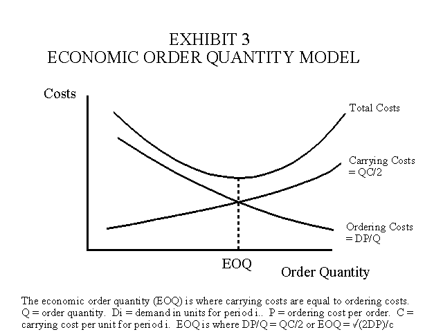
Example: Assume demand per period is Di = 112,500 units, ordering costs per purchase order is P = $100, carrying cost per unit per period i is C = $10. Then the EOQ is found by equating ordering costs with carrying costs as follows: (112,500)(100)/Q = (Q)(10)/2. Then 11,250,000/Q = Q5 and 2,250,000 = Q². Take the square root and the EOQ = 1,500 units.

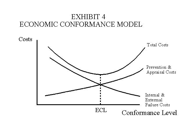
5. The quality cost conformance model provides another example of a constrained optimization approach. In this model the economic conformance level (ECL) is obtained where prevention and appraisal costs are equal to external and internal failure costs. Prevention and appraisal costs increase as the level of conformance quality increases. Conformance quality refers to conformance to specifications as opposed to design quality. Failure costs are expected to decrease as the level of conformance quality increases. Therefore, the total costs associated with conformance quality will be U-shaped as indicated in Exhibit 4. The optimization concept and related calculations are essentially the same as in the EOQ model. Prevention costs include quality engineering, training and related supervision costs. Appraisal costs include inspection, testing and supervision related to these activities. Internal failure costs include spoilage, scrap, rework and the associated downtime costs, while external failure costs include warranty costs and the costs of lost customers.

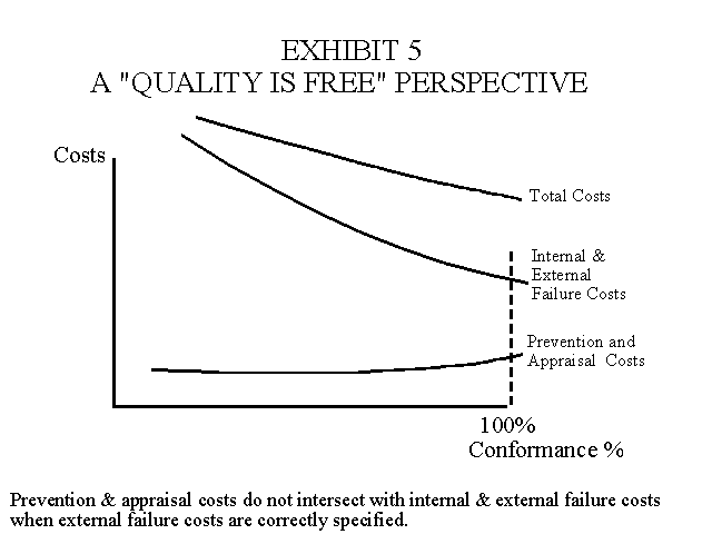
The ECL model is associated with Juran. Deming and others, such as Crosby (Quality Is Free: The Art of Making Quality Certain) view the calculation of the ECL as a waste of time. From this perspective, the main problem with the ECL methodology is that the model is likely to be mis-specified by underestimating or ignoring the costs associated with lost customers. A revised model with the "quality is free" perspective is provided in Exhibit 5. This is a long run view where the lost sales dollars resulting from past failures are included in external failure costs. Of course, lost sales dollars are unknown amounts, but there is adequate reason in most industries to believe that they represent substantial amounts, perhaps so large that the two curves never intersect.

Quality Models Compared

Two quality models have appeared in the accounting literature in recent years. Juran's quality cost conformance model is associated with the zero defect philosophy shown on the left side in the illustration below. Juran's model includes a target value and tolerance, or specification limits, for the variation that occurs in a parameter or characteristic (X). In Juran's model, no loss occurs if the value of X is within the specification limits, i.e., it is considered acceptable. If the value is outside the limits it is considered unacceptable or a defect and becomes either scrap, spoilage or rework.

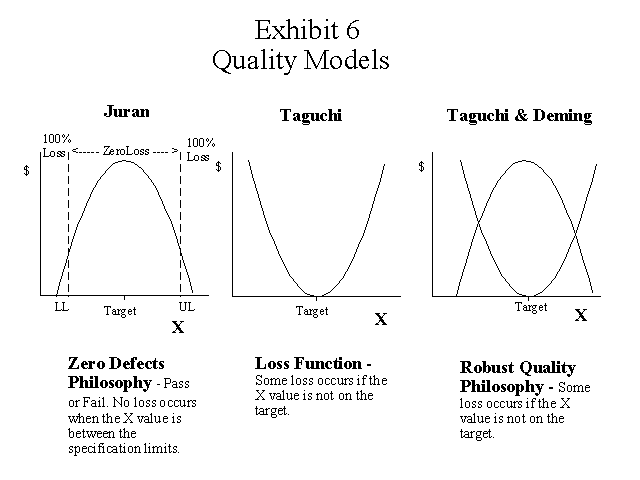
Deming, on the other hand, was associated with the robust quality philosophy based on Taguchi's loss function shown in the center of the illustration and combined with a distribution of X on the right hand side. Taguchi and Deming believed that some loss occurs for the manufacturer, the customer, or society when the value of X is not on target. In the graphic illustration above, the distribution of X is drawn so that it appears that the mean of X is on the target value, but of course this is not usually the case. The idea in the robust quality philosophy is to continuously improve the process by moving the mean value of the parameter closer to the target value and by reducing the amount of variation in the parameter.

6.Relevant cost (incremental, differential or cost-benefit) models such as special order pricing decisions, product mix decisions, make or buy (out-sourcing) decisions, to process joint products further decisions and similar short term decisions all fall into the constrained optimization category because a static environment is typically assumed. Some relevant cost problems, such as the product mix decision model, use techniques such as linear programming because there are a large number of constraints that must be considered simultaneously.

7. The conventional capital budgeting investment decision model. This model is essentially a long run relevant cost model that emphasizes the discounted cash flow methodology, i.e., net present value and internal rate of return approaches. It falls into the constrained optimization category because a static environment is typically assumed. The investment management concept adds the moving baseline approach to the model to make it more dynamic.

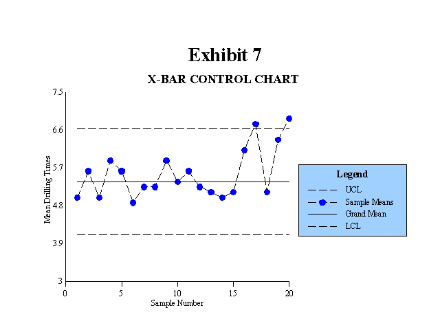
8. The statistical process control (SPC) model might also be included in the constrained optimization category from the perspective that it measures the variability within a stable or static system. However, sample means that fall outside the control limits indicate that the system is no longer stable. Changes in the system that cause changes in the mean or changes in the range are also reflected on the control charts. This adds a dynamic element to the SPC methodology that makes it useful as a tool for measuring improvements in the system. A system improvement represents a change that either improves the mean outcome or reduces the variability within the system. For the illustration in Exhibit 7, a change in the production process that reduced the mean drilling time or reduced the variability in drilling time would represent a system improvement.

9. Converting static models into dynamic models. In defense of the constrained optimization techniques, one can argue that all of the methods discussed above can be converted into dynamic, rather than static models by adding sensitivity analysis to the model. Sensitivity analysis involves testing how sensitive the solution is to changes in the constraints associated with the model. For example, sensitivity analysis is frequently used in product mix decisions based on linear programming. One can also argue that ignoring potential improvements in the system when using a model does not represent a flaw in the model, but instead indicates a myopic misuse of the model. A rebuttal is that most users may ignore the sensitivity issue because it is not a formal part of the model.

___________________________________________

¹ Martin, J. R. 1994. A controversial-issues approach to enhance management accounting education. Journal of Accounting Education 12(1): 59-75. (Summary).

Other related summaries:

Albright, T. L. and H. Roth. 1992. The measurement of quality costs: An alternative paradigm. Accounting Horizons (June): 15-27. (Summary).

Albright, T. L. and H. P. Roth. 1994. Managing quality through the quality loss function. Journal of Cost Management (Winter): 20-37. (Summary).

Anderson, S. W. and K. Sedatole. 1998. Designing quality into products: The use of accounting data in new product development. Accounting Horizons (September): 213-233. (Summary).

Deming, W. E. 1993. The New Economics For Industry, Government & Education. Massachusetts Institute of Technology Center for Advanced Engineering Study. (Summary).

Goldratt, E. M. 1990. What is this thing called Theory of Constraints. New York: North River Press. (Summary).

Johnson, H. T. 1989. Professors, customers, and value: bringing a global perspective to management accounting education. Proceedings of the Third Annual Management Accounting Symposium. Sarasota: American Accounting Association: 7-20. (Summary).

Johnson, H. T. 1992. Relevance Regained: From Top-Down Control to Bottom-up Empowerment. The Free Press. (Summary).